Control Systems – Electrical Engineering Optional PYQs (1995–2026)

Here are all 186 Control Systems questions asked in UPSC Electrical Engineering Optional Paper II from 1995 to 2026, arranged under the 6 topics of the official syllabus. Within each topic the latest questions come first.

Each question ends with a code such as [2024/15m/3b] – the year, the marks, the word limit (where UPSC set one) and the question number in the paper.

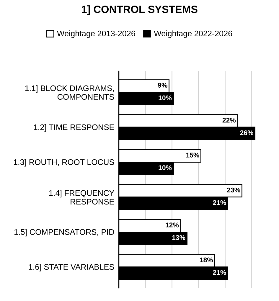
1.1] Control system basics and block diagrams

31 questions

1. The block diagram of a system is as shown below: Evaluate the overall transfer function $\frac{Y\left(s\right)}{R\left(s\right)}$ using block diagram reduction technique.

[Figure: $R\left(s\right)$ is picked off to two paths: (1) through block $G_3$ to the third summing junction (+ input); (2) to the first summing junction (+). First summing junction output → $G_1$ → second summing junction (+) → pick-off point P → $G_2$ → third summing junction (+) → $Y\left(s\right)$. Feedback $H_1$: from $Y\left(s\right)$ through block $H_1$ to the second summing junction (− input). Feedback $H_2$: from point P (output of the second summing junction, before $G_2$) through block $H_2$ to the first summing junction (− input); this line crosses the $H_1$ feedback line without connection] [2025/10m/1a]

2. The signal flow graph of a system is as shown below: Determine the overall transmission $\frac{R\left(s\right)}{Y\left(s\right)}$, and evaluate the sensitivity of the output to variations in $K_1$ at $s=10$. What would be the value of sensitivity obtained under DC condition, i.e., $s=0$?

[Figure: Signal flow graph with nodes $R\left(s\right)$, $x_1$, $x_2$, $x_3$, $x_4$, $x_5$, $Y\left(s\right)$. Forward branches: $R\left(s\right)\to x_1$ gain 1; $x_1\to x_2$ gain 2; $x_2\to x_3$ gain $K_1$; $x_3\to x_4$ gain $\frac{1}{s(s+2)}$; $x_4\to x_5$ gain $\frac{1}{s}$; $x_5\to Y\left(s\right)$ gain 1. Self-loop at $x_5$ with gain 1. Feedback branches: $x_3\to x_1$ gain −1; $x_5\to x_3$ gain −2; $x_5\to x_1$ gain −1] [2025/10m/3a(ii)]

3. The block diagram of a position control system is shown in the figure. Determine the sensitivity of the closed loop transfer function T(s) with respect to G(s) and H(s) for 1 rad/sec.

[Figure: Negative feedback loop: $R\left(s\right)$ enters a summing junction (+); its output feeds the forward block $G\left(s\right)=\frac{10}{s(s+1)}$ whose output is $C\left(s\right)$; $C\left(s\right)$ is fed back through the block $H\left(s\right)=5$ to the − input of the summing junction.] [2024/10m/5a]

4. Determine the transfer function $C\left(s\right)/R\left(s\right)$ for the signal flow graph of the system shown below using Mason’s gain formula:

[Figure: Signal flow graph with nodes $x_1$ (input $R\left(s\right)$) to $x_6$ (output $C\left(s\right)$) in a line. Forward branches: $x_1\to x_2$: $G_1\left(s\right)$; $x_2\to x_3$: $G_2\left(s\right)$; $x_3\to x_4$: $G_3\left(s\right)$; $x_4\to x_5$: $G_4\left(s\right)$; $x_5\to x_6$: unlabelled (unity). Self-loop at $x_2$ with gain −1. Feedback branches from $x_5$: to $x_4$ gain −1; to $x_3$ gain −1; to $x_2$ gain −1.] [2022/10m/4c]

5. For the network shown in figure, draw a block diagram representing each circuit element by a block. Use block diagram reduction technique to obtain the transfer function of the network. The voltage $V_i\left(t\right)$ is the applied input and the voltage across the capacitor $V_o\left(t\right)$ is the output.

[Figure: Ladder RC network: input $V_i\left(t\right)$ (+ at top); current $I_1\left(t\right)$ through series $R_1$ to node $V_1\left(t\right)$; capacitor $C_1$ from $V_1\left(t\right)$ to the bottom (return) line; current $I_2\left(t\right)$ through series $R_2$ from $V_1\left(t\right)$ to the output node; capacitor $C_2$ from the output node to the bottom line, output $V_o\left(t\right)$ across $C_2$ (+ at top).] [2021/20m/2b]

6. Find the transfer function X(s)/E(s) for the electromechanical system shown in the following figure. Consider (1) the force acting on mass $P\left(t\right)=K_2{i}_2\left(t\right)$ and (2) the back e.m.f. of coil $e_b\left(t\right)=K_1\frac{dx\left(t\right)}{dt}$, where $K_1$ and $K_2$ are constants.

[Figure: Electromechanical system: input voltage e(t) applied at the left terminals; series resistor R from the upper input terminal to a node; capacitor C from that node to the lower (return) wire; from the node, series inductor L to a coil whose other end returns to the lower wire; mesh currents $i_1\left(t\right)$ (left mesh, through R and C) and $i_2\left(t\right)$ (right mesh, through C, L and the coil), both drawn clockwise; the coil (back e.m.f. $e_b\left(t\right)$) is wound on a plunger that exerts force P(t) on mass M; M is connected to a fixed wall through a spring K and a damper D in parallel; displacement x(t) of M measured to the right] [2019/10m/4a(i)]

7. The block diagram representation of a control system is shown below:

[Figure: Two-input two-output block diagram. Summing junction 1: $R_1$ (+) and feedback $H_1$ (+), where $H_1$ is fed from output $C_2$; its output $E_1$ feeds blocks $G_1$ and $G_3$. Summing junction 2: $R_2$ (+) and feedback $H_2$ (+), where $H_2$ is fed from output $C_1$; its output $E_2$ feeds blocks $G_4$ and $G_2$. Output summing junction for $C_1$: $G_1$ output (+) and $G_4$ output (+), giving $C_1$. Output summing junction for $C_2$: $G_3$ output (+) and $G_2$ output (+), giving $C_2$]

Find $\frac{C_2}{R_1}$ transfer function using the following: (1) Block diagram reduction method (2) Mason’s gain formula [2019/10m/4a(ii)]

8. For the block diagram shown in the figure given below, obtain $\frac{C\left(s\right)}{R\left(s\right)}$ using block diagram reduction technique:

[Figure: Block diagram: R(s) → block $1/s$ → summing junction 1 (this signal enters with +) → block $1/s$ → summing junction 2 (this signal enters with +) → C(s). A feedforward line drops from the underside of the first $1/s$ block, runs along the bottom and enters summing junction 1 from below (no sign printed) and summing junction 2 from below (sign +)] [2015/10m/1a]

9. Using the Block diagram simplification method reduce the block diagram of the following control system to a block diagram of the following type:

[Figure: Given block diagram: R(s) enters summing junction 1 (+); its output goes to summing junction 2 (+), then through block 10 and block $\frac{1}{s+1}$ in cascade to a take-off point X. From X: (1) through block $\frac{1}{s}$ to summing junction 3 (+ input from the left); (2) through an upper parallel block 10 to summing junction 3 (+ input from the top); (3) through a feedback block s back to summing junction 2 (– input). The output of summing junction 3 is C(s), which is fed back directly (unity) to summing junction 1 (– input).]

[Figure: Required form: R(s) to a summing junction (+), forward block G(s) giving C(s), feedback block H(s) from C(s) back to the summing junction (– input).] [2013/20m/2a]

10. .

(i) Some control systems have more than one inputs applied at different points in the system. How do we find the response of such systems, using block diagram algebra? Illustrate your answer with the help of a simple example. [2012/10m/4c(i)]

(ii) For the block diagram representation of the figure shown below, determine the system characteristic equation. Is the system represented by this block diagram stable?

[Figure: $R\left(s\right)$ → summing junction (+) → forward block $(s+1)(s+3)$ → $C\left(s\right)$; feedback from $C\left(s\right)$ through block $\frac{1}{(s+2)(s+4)}$ to the (−) input of the summing junction] [2012/10m/4c(ii)]

11. For the block diagram shown in the figure below, find the overall transfer function of the system. Verify the same, using signal-flow graph analysis:

[Figure: $R\left(s\right)$ → summing junction 1 (+ for R(s), − for feedback) → $G_1$ → summing junction 2 (+ from $G_1$, − from feedback) → $G_2$ → node 3 → $G_3$ → node 4 → $C\left(s\right)$. Feedback from node 3 through $H_1$ to the (−) input of junction 1; feedback from node 4 through $H_2$ to the (−) input of junction 2] [2012/20m/6c]

12. The diagram of a speed control system is given below: The generator e.m.f. $e_g$ is 2000 volts per field ampere. The motor e.m.f. $e_m$ is 1.5 volts ${rad}^{-1}$ sec. The motor torque $K_T$ is 0.5 N m per armature ampere and the inertia of motor and load is ${10}^{-4}kg{m}^2$. Assuming negligible friction, determine the transfer function $\frac{\omega \left(s\right)}{V_{in}\left(s\right)}$.

[Figure: Generator field circuit: input voltage $V_{in}$ applied across a 100 Ω resistor in series with a 1H field inductance. Armature loop: generator armature (e.m.f. $e_g$) connected through a 100 Ω resistor to the motor armature (e.m.f. $e_m$), the lower terminals of the two machines joined directly. The motor shaft (speed $\omega$) drives the load of inertia J] [2011/20m/2a]

13. A model of the attitude control of a space booster on take off is represented by an inverted pendulum mounted on a motor driven cart shown in the above figure. The objective of the attitude control problem is to keep the pendulum in a vertical position. The pendulum can be assumed to move only in one plane (say the $xy$ plane). The control force ‘$u$’ is applied to the cart. The centre of gravity of the pendulum is at its centre. The moment of inertia of the pendulum is ‘$I$’. The mass of the pendulum is ‘$m$’ and the cart is ‘$M$’. Obtain a mathematical model.

[Figure: (printed above the text) Inverted pendulum on a cart: cart of mass M on wheels on a horizontal floor (x-axis to the right), a fixed wall at the left forming the y-axis; horizontal distance x measured from the wall (y-axis) to the pivot of the pendulum on top of the cart; pendulum (rod) pivoted on the cart, tilted to the right by angle $\theta$ from the vertical; total length $2l$ marked as $l$ from the pivot to the centre and $l$ from the centre to the top; weight $mg$ acting downward at the centre; height of the centre above the pivot marked $lcos\theta$; control force $u$ applied horizontally to the cart (arrow to the right); x-direction arrows at the cart top and at the floor] [2010/20m/5a]

14. Determine the transfer function of the network shown in Fig.:

[Figure: Fig. – Two-section RC ladder: input $V_i$ (+ at top) – series $R_1$ – node – shunt $C_1$ to the common bottom line – series $R_2$ – node – shunt $C_2$ to the bottom line; output $V_o$ (+ at top) taken across $C_2$] [2009/20m/1a]

15. State and explain the Mason’s Gain formula. Determine all input-output relationships of the system represented by the set of following linear equations using the Mason’s Gain formula: $x_1=a_{11}{x}_1+a_{12}{x}_2+b_1{u}_1$, and $x_2=a_{21}{x}_1+a_{22}{x}_2+b_2{u}_2$ where $u_1$ and $u_2$ are the inputs and $x_1$ and $x_2$ are the states of the system. [2005/20m/2a]

16. Describe the working of a stepper motor. [2004/5m/1c(ii)]

17. Explain the effects of negative feedback in control systems on the following (i) Stability (ii) External disturbances. [2003/20m/2a]

18. Show that the feedback reduces the effect of parameter variation on the performance of the control system, but adversely affects the gain of the systems Also discuss briefly the effect of feedback on the transient performance of the control system. [2002/20m/7a]

19. Describe the constructional features and working of a 2-phase, 4/6 pole hybrid stepping motor. Discuss its torque-displacement characteristics also. [1999/20m/8a]

20. Select any Three of the following statements, read them carefully and identify correct and incorrect ones. Justify your answer using not more than 200 words in each case: In analog simulation of physical system, Integrators are used rather than Differentiators. [1998/20m/200w/1a]

21. Select any Three of the following statements, read them carefully and identify correct and incorrect ones. Justify your answer using not more than 200 words in each case: Synchro error detectors are used in dc servo system. [1998/20m/200w/1c]

22. Discuss briefly the speed-torque characteristics of a 2$\varphi$ ac servomotor and compare it with that of ordinary 3$\varphi$ induction motor. Hence describe the laboratory method to obtain its speed-torque characteristic. [1998/20m/2b]

23. Describe with the help of a neat diagram the operation of a reluctance-type stepper motor along with its characteristics. What are its possible applications? [1998/20m/8b]

24. Select any three of the following statements, read them carefully and identify the correct and the incorrect ones. Justify your answer using not more than 200 words in each case. A two-phase a.c. Servomotor is similar in all respects to a conventional induction motor. [1997/20m/200w/1b]

25. A system is represented by the following equations: $x=x_1+3u$ $x_1=-3x_1+x_2+2u$ $x_2=-2x_1+u$ Find the transfer function $\frac{X\left(s\right)}{U\left(s\right)}$ by signal flow technique. [1997/20m/2b]

26. Give the schematic of two synchro pairs, one pair being useful for remote control and the other pair functioning as a transducer for converting angular position into an electrical signal. [1996/10m/1d(i)]

27. Distinguish between open-loop and closed-loop system. Convert the system of Fig. 1 into a unity feedback system.

[Figure: Fig. 1: Block diagram: input R enters summing point 1 (+); its output splits into two parallel paths, one through block $\frac{1+j\omega }{1+0.5j\omega }$ and the other through block 10, which are added at summing point 2 (both +); the sum passes through block $\frac{6}{{\left(j\omega \right)}^2}$ [?] to the output C; C is fed back through block 3 [?] to summing point 1 (−)] [1996/20m/2b]

28. What is a servomotor? Give the characteristics of a 2-phase servomotor and obtain its transfer function. A 50 Hz, 2-phase, ac. servomotor has the following parameters: Starting torque = 0.186 N-m Rotor inertia = $1\times {10}^{-5}kg{m}^2$ Supply voltage = 120 V No-load angular velocity = 304 rad/sec Assuming straight line torque-angular speed characteristics of the motor and zero viscous friction derive the transfer function. [1996/20m/3b]

29. Give the constructional features, principle of operation and applications of a variable reluctance stepper motor. [1996/20m/7b]

30. The forward path transfer function of a position control system with velocity feedback is given by $G\left(s\right)=\frac{K}{s(s+p)}$ Determine the sensitivity of the transfer function of the closed-loop system to changes in K, p and a for transfer function of the feedback path (i) $H\left(s\right)=1$, and (ii) $H\left(s\right)=(1+\alpha s)$. The nominal values of the parameters are $K=12$, $p=3$ and $\alpha =0.14$. [1995/20m/2b]

31. What are Tachogenerators? Discuss with block diagram, their application to closed-loop control systems. [1995/20m/3a]

1.2] Time-domain and transform-domain analysis

39 questions

1. A unity feedback system has open loop transfer function $G\left(s\right)=\frac{K}{s(s+q)}$. Evaluate the value of $K$ and $q$ so that settling time and peak overshoot will be 6 seconds and 20% respectively. [2026/10m/1a]

2. Determine the response of the system shown in the following figure when it is excited by a unit step input.

[Figure: Unity negative feedback loop: $R\left(s\right)$ enters a summing junction (+); the junction output passes through block $s+1$ and then block $\frac{2}{s^2}$ in cascade to give $C\left(s\right)$; $C\left(s\right)$ is fed back directly (unity feedback) to the summing junction with − sign] [2026/20m/2a]

3. A system has a unit response as $c\left(t\right)=1-e^{-0.5t}$. Evaluate its unit impulse and unit ramp response, assuming zero initial conditions. [2026/10m/3a(i)]

4. Consider a second-order type-1 system with no zeros. The system under unity feedback admits a resonant peak of 1.36 at resonant frequency 8.2 rad/s. Compute the transfer function $G\left(s\right)$, and its steady-state error due to input signal $x\left(t\right)=2u\left(t\right)+3t\cdot u\left(t\right)$ under unity feedback. [2025/10m/4a(i)]

5. Given a second-order linear time-invariant system $G\left(s\right)$ with a relative degree of 2. $G\left(s\right)$ admits a zero steady-state error for unit step input and steady-state error of 0.1 for unit ramp input under unity feedback configuration. Further, it admits a settling time of 4 seconds for 2% tolerance band in its unit step response under unity feedback. A delay of $T$ seconds is now placed in cascade with $G\left(s\right)$. Calculate the value of $T$ in seconds that will make the delayed system oscillate under unity feedback configuration. [2025/10m/5a]

6. The first order system and its response to unit step input are shown in Figure I and II respectively. Determine the system parameters ‘a’ and ‘K’.

[Figure I: Block diagram: input $u\left(t\right)$ → block $\frac{K}{s+a}$ → output $c\left(t\right)$.]

[Figure II: Unit-step response $c\left(t\right)$ versus Time (t) (in sec): an exponential rise from 0 approaching a final value of 2.0 (dashed horizontal line); the dashed tangent to the curve at the origin meets the 2.0 line at $t=0.2$ (dashed vertical line at 0.2).] [2024/10m/4c]

7. The figure shows a unity feedback system. The steady-state value of the unit step response $c\left(t\right)$ is 0.8. Determine the maximum overshoot in the response $c\left(t\right)$:

[Figure: Unity negative feedback loop: input $u\left(t\right)$ to a summing junction (+), forward block $\frac{K}{(s+1)(s+2)}$, output $c\left(t\right)$ fed back directly to the − input of the summing junction.] [2023/10m/1a]

8. Find the value of $R$ so that the system shown in the figure is critically damped. $V_i\left(t\right)$ is the input voltage and output $V_o\left(t\right)$ is the voltage across the capacitance. $L=90\mu H$, $C=120nF$:

[Figure: Series R–L from the input terminal to the output node; capacitor $C$ from the output node to the common bottom line; input $V_i\left(t\right)$ on the left, output $V_o\left(t\right)$ across $C$.] [2023/10m/6c]

9. A closed-loop system is shown in the figure below. The maximum overshoot for the system is 40% and the peak time is 2 seconds. Calculate the values of A and B. Consider $J=1kg\mathrm{\text{–}}{m}^2$:

[Figure: Block diagram: $R\left(s\right)$ enters summing junction 1 (+); its output enters summing junction 2 (+); its output passes through block $\frac{A}{Js}$ and then block $\frac{1}{s}$ to the output $C\left(s\right)$. The signal at the output of $\frac{A}{Js}$ (before $\frac{1}{s}$) is fed back through block B to the − input of summing junction 2. The output $C\left(s\right)$ is fed back with unity gain to the − input of summing junction 1.] [2022/10m/1a]

10. A unity feedback system is shown in the figure below. Determine the range of $\alpha$ for which the system is stable and the steady-state error for unit step input is less than 5%:

[Figure: Unity negative feedback loop: $R\left(s\right)$ enters a summing junction (+), the output $C\left(s\right)$ is fed back to its − input; forward path block $\frac{s+\alpha }{s^3+(1+\alpha )s^2+(\alpha -1)s+(1-\alpha )}$.] [2022/20m/2a]

11. The unit impulse response of a linear system is given by $c\left(t\right)=e^{t}u\left(t\right)+e^{-t}u\left(t\right)$. When the same system is subjected to an input of $e^{-3t}u\left(t\right)$, determine the output of the system. Assume that the system is initially relaxed. [2020/10m/5a]

12. The overall transfer function of a control system is given by $\frac{C\left(s\right)}{R\left(s\right)}=\frac{16}{(s^2+1.6s+16)}$ It is desired that the damping ratio be 0.8. Determine the derivative rate of feedback constant $K_d$, and compare rise time, peak time, maximum overshoot and steady-state error for unit ramp input without and with derivative feedback control. [2019/20m/7a]

13. For the system, whose open-loop transfer function is $G\left(s\right)H\left(s\right)=\frac{K}{{(s+2)}^2(s+3)}$, determine $K$ which satisfies the following specifications: (i) Position error constant $K_p\ge 2$ (ii) Gain margin $\ge 3$ [2018/20m/3b]

14. Consider a unity feedback control system whose forward path transfer function is given by $G\left(s\right)=\frac{9}{s(s+1)}$. Determine–.

(i) percentage overshoot resulting from application of unit step input; [2018/10m/4a(i)]

(ii) steady-state error resulting from application of unit step and unit ramp input. [2018/10m/4a(ii)]

15. Consider a unity feedback system having transfer function $\frac{C\left(s\right)}{R\left(s\right)}=\frac{a}{s^2+bs+a}$. Determine the open-loop transfer function and steady state error coefficients. [2017/15m/4b]

16. For $\gamma \left(t\right)=0.9t$, it is required that the steady state error should be less than 0.05. Determine the value of gain (K) of proportional controller for the system shown above.

[Figure: (printed above the question text) Unity negative feedback system: R(s) enters a summing junction (+), the feedback enters with (−); the error passes through a block K and then a block $\frac{1}{s(s+2)}$ to give the output C(s); C(s) is fed back directly (unity feedback) to the summing junction] [2017/10m/5e]

17. (i) Figure 2(a) shows the block diagram of a control system. Find its characteristic equation. (ii) Calculate its damping factor and undamped natural frequency for K = 10. (iii) What should be the value of K for critical damping? (iv) For K = 10, find the expression for c(t) and obtain the time at which the first overshoot occurs. Also calculate the peak overshoot magnitude.

[Figure: Figure 2(a): Block diagram: R(s) → summing junction 1 (R(s) with +, outer feedback with −) → summing junction 2 (+ from junction 1, − from inner feedback) → forward block $\frac{K}{s(s+2)}$ → C(s). Inner feedback: from C(s) through a block $0.25s$ back to the − input of junction 2. Outer feedback: unity, from C(s) back to the − input of junction 1] [2016/20m/2a]

18. Explain the following terms in reference to performance indices in a control system: 1. Rise time 2. Integral square error 3. Integral of time multiplied square error 4. Integral absolute error 5. Integral of time multiplied absolute error. [2016/10m/8a(i)]

19. A system input (x)-output (y) is described by the relation $\frac{d^{2}y}{d{t}^2}+8\frac{dy}{dt}+ky=50x\left(t\right)$ Evaluate the response $y\left(t\right)$ and its maximum value for an input $x\left(t\right)=2.5u\left(t\right)$, $u\left(t\right)$ is a unit step function. Given $k=25$. [2015/10m/1b]

20. Draw the approximate time response of an underdamped second order system subjected to unit step input disturbance in desired value for the following cases of complex conjugate poles: (i) with constant real part (ii) with constant imaginary part (iii) with constant damping ratio In each case consider at least 2 sets of values and mention the most important feature of the response. [2014/20m/3a]

21. State and explain various test inputs in control systems. [2013/10m/1e]

22. For the control system: the steady state error for unit ramp input is 0.01. Determine the value of K.

[Figure: Unity negative feedback system: R(s) to a summing junction (+), forward block $\frac{K}{s(sJ+f)}$ giving C(s); C(s) fed back directly to the summing junction (– input). Data beside the figure: $f={10}^{-1}$ Newton m per rad/sec; $J=5\times {10}^{-3}kg\mathrm{\text{–}}{m}^2$.] [2013/5m/5a(ii)]

23. Identify the correctness of the following statements. Justify your answers:

(i) The root locus gives idea about system’s transient behaviour. [2012/3m/1a(i)]

(ii) For an inherently stable second-order system, all the coefficients of characteristic equation are of the same sign. [2012/4m/1a(ii)]

(iii) A critically damped system has sustained oscillations. [2012/3m/1a(iii)]

24. For the control system, shown in the following figure, determine the steady-state error for a unit step input in terms of $K$ and $K_1$, where $E\left(s\right)=R\left(s\right)-C\left(s\right)$. Determine the value of $K_1$, when steady-state error is zero:

[Figure: Block diagram: $R\left(s\right)$ → block $K_1$ → summing junction (+ from $K_1$, − from feedback); its output $E\left(s\right)$ → block $\frac{K}{s(s+10)(s+12)}$ → $C\left(s\right)$; unity negative feedback from $C\left(s\right)$ to the summing junction] [2012/20m/2a]

25. Consider the system shown in Fig. 6(a) where the damping ratio $\xi =0.6$ and the natural frequency ${\omega }_n=5$ rad/sec. Obtain the values of rise time $t_r$, peak time $t_p$, maximum overshoot $M_p$ and settling time $t_s$ for the 2% criterion when the system is subjected to a unit-step input.

[Figure: Fig. 6(a) – Unity negative feedback loop: R(s) enters a summing junction (+), whose output feeds the forward block $\frac{{\omega }_n^2}{s(s+2\xi {\omega }_n)}$ giving C(s); C(s) is fed back directly to the (−) input of the summing junction] [2009/20m/6a]

26. Select any three of the following statements, read them carefully and identify the correct and the incorrect ones. Justify your answer using not more than 200 words in each case The steady – state errors for unit step input to type-0, type-1 and type-2, unity feedback systems are finite non-zero, zero and infinite respectively. [2002/20m/200w/5a]

27. Determine the output c(t) at t = 2 sec for the system shown in the above figure.

[Figure (printed above the text): Sampled-data unity-feedback system: unit step input to a summing junction (+ input; − feedback from the output c(t)); error passes through a sampler with T = 1 sec, then a ZOH block, then a plant block $\frac{1}{s+2}$, whose output is c(t). “ZOH: Zero Order Hold”.] [2000/20m/8a]

28. Select any three of the following statements, read them carefully and identify the correct and the incorrect ones. Justify your answer using not more than 200 words in each case. Feedback provides same control on the steady state error to standard inputs by adjustment of open-loop gain. [2000/20m/200w/5a]

29. What is Bode-plot? Discuss how a Bode-plot can be drawn. Derive the step response of a second order system expressed by: $a\frac{d_2\theta }{dt}+b\frac{d\theta }{dt}+c\theta =F\left(t\right)$. [1999/20m/2a]

30. The pole-zero configuration of a closed-loop control system is given by $(s_1,s_2)=-2\pm j2$. Calculate the undamped resonance frequency and the damping ratio. [1999/10m/2c(i)]

31. The roots of a second order system are located at $-1+j2$ and $-1-j2$. Determine the followings if the system is excited by unit step input: (i) Damping ratio (ii) Maximum % overshoot (iii) Natural frequency of oscillation (iv) Damped frequency of oscillation. [1998/20m/2a]

32. The unity feedback system has forward path transfer function $G\left(s\right)=\frac{S+1}{s^2(s+2)(s+4)}$ Determine steady state error coefficients $K_p$, $K_v$ and $K_a$. Hence find the steady state error in output if (i) unit step input, (ii) unit ramp input and (iii) unit parabolic input are given. [1998/20m/3b]

33. Sketch the under-damped time response of a second order control system to a step input. Define clearly the “Delay time”, “Rise time”, “Peak time”, “Peak-overshoot”, “Settling time” and “Steady state error” and also show them in the sketch. [1997/20m/2a]

34. The response of an initially relaxed time invariant constant parameter system to a unit impulse applied at $t=0$ is $4e^{-2t}u\left(t\right)$. (i) Find through time domain analysis the response to the same system to an input $e^{-t}u\left(t\right)$ (ii) Find the time function which when applied to the system would yield a response $sin2t.u\left(t\right)$. [1997/20m/3a]

35. An open loop transfer function of unity feedback system is given by $G\left(s\right)=\frac{25}{s(s+2)}$. Determine the damping factor, undamped natural frequency, damped natural frequency and time response for a unit step input. [1997/20m/3b]

36. Select any three of the following statements, read them carefully and identify the correct and incorrect ones. Justify your answer using not more than 200 words in each case. By adding a pole to the closed loop transfer function, the maximum overshoot increases and the effect is opposite to that of adding a pole to the open loop transfer function. [1996/20m/200w/1b]

37. Describe a simple position control system. A certain position control system is driven by $100:1$ gear by a motor whose torque characteristics is of the form $(10V_m-0.3N){10}^{-4}$ N-m, where N is the speed in R.P.M. and is the voltage supplied by the amplifier. If the synchros produce 1 V/ degree error and if the steady state error should be 5° for a speed input of 20 RPM, calculate the required amplifier gain. Viscous friction at the motor shaft is $60\times {10}^{-6}$ Nm-sec. [1996/20m/2a]

38. Select any three of the following statements, read them carefully and identify the correct and incorrect ones. Justify your answer using not more than 200 words in each case. Knowing the step response of a system the response to a ramp input cannot be deduced. [1995/20m/200w/1b]

39. The block diagram of an electronic pacemaker is given in Fig 1, where $K=400$. (i) Calculate the output c(t) for a unit step input. (ii) Calculate the integral of the square of the error between input and the output. (iii) Determine the steady-state error for a unit ramp input. (iv) Determine the value of K for which the steady-state error to a unit ramp will be 0.02.

[Figure: Fig. 1: Unity negative feedback loop: input r(t) (“Desired heart rate”) enters a summing point (+); its output passes through the “Pacemaker” block $\frac{K}{s+20}$ and then the “Heart” block $\frac{1}{s}$ to give the output c(t) (“Actual heart rate”); c(t) is fed back directly to the summing point (−)] [1995/20m/3b]

1.3] Stability: Routh–Hurwitz and root locus

33 questions

1. Sketch the approximate root locus plot for a time-delay system approximated by the transfer function $G\left(s\right)=\frac{K(1-\frac{s}{2})}{s(s+1)(1+\frac{s}{2})}$ Also compute the largest value of $K$ for which the system is stable under unity feedback. Verify this value from the root locus plot. [2025/10m/3a(i)]

2. The block diagram of a feedback system is shown in the figure. (i) Sketch the complete root locus of the system. (ii) What is the value of $K$ at $s=0$? (iii) Find the range of $K$ for closed-loop stability.

[Figure: Negative feedback loop: $R\left(s\right)$ to a summing junction (+); forward block $\frac{K}{(s-1)(s^2+4s+7)}$ with output $C\left(s\right)$; feedback block $s+4$ from $C\left(s\right)$ to the − input of the summing junction.] [2023/20m/2a]

3. A unity feedback system is shown in the figure below. Determine the range of $\alpha$ for which the system is stable and the steady-state error for unit step input is less than 5%:

[Figure: Unity negative feedback loop: $R\left(s\right)$ enters a summing junction (+), the output $C\left(s\right)$ is fed back to its − input; forward path block $\frac{s+\alpha }{s^3+(1+\alpha )s^2+(\alpha -1)s+(1-\alpha )}$.] [2022/20m/2a]

4. The two top rows of a Routh table of a characteristic polynomial is given in the table. Determine the roots of the characteristic equation which lie in the left half s-plane. Complete the remaining rows of the table.

$s^4$	1	10	24
$s^3$	5	20

[2021/10m/5b]

5. The open-loop transfer function of a feedback system is given by $G\left(s\right)H\left(s\right)=\frac{K(s+3)}{(s-1)(s-2)}$. Determine the gain K at the break-in point of the root locus of the system. [2020/10m/1a]

6. The unit step response of a unity feedback system exhibits sustained oscillations as shown in the figure below. The open-loop transfer function of the system is $G\left(s\right)=\frac{K}{(s+1)(s+4)(s+a)}$. The time x in the figure is 1.0471 second. Determine the values of K and a.

[Figure: Unit step response against Time (second), axis marked 0, 2, 4, 6: starting from zero at t = 0, a sustained (undamped) sinusoidal oscillation about a horizontal dash-dot line (the mean level), with peaks near t ≈ 1.2, 3.3 and 5.4 s and minima near t ≈ 2.2 and 4.3 s; the interval x is marked on the dash-dot line between the first upward crossing of the mean level and the next downward crossing (half a period)] [2020/20m/2a]

7. Sketch the root locus from the open-loop transfer function $G\left(s\right)H\left(s\right)=\frac{K}{s(s+6)(s^2+4s+13)}$ and determine the following: (i) The angles of departure from complex poles (ii) The break-away points (iii) The intersection with imaginary axis (iv) The stability conditions. [2019/20m/3b]

8. A unity feedback control system is characterized by the open-loop transfer function $G\left(s\right)=\frac{K(s+13)}{s(s+3)(s+7)}$ (i) Using the R-H criterion, calculate the range of values of K for the system to be stable. (ii) Check whether for K = 1, all these roots of the characteristic equation of the above system have damping factor greater than 0.5. [2019/10m/5e]

9. For the open-loop transfer function $G\left(s\right)H\left(s\right)=\frac{K}{s(s+4)(s+5)}$, determine the following: (i) Point of intersection of asymptotes with real axis (ii) Point of intersection of root locus with imaginary axis and the value of $K$ at this point. [2018/10m/1c]

10. The characteristic equation of a system is given by $s^4+3s^3+10s^2+20s+100=0$ By Routh-Hurwitz criterion, determine the number of poles of the system with positive real parts. [2018/10m/5e]

11. For the open-loop transfer function $G\left(s\right)H\left(s\right)=\frac{K(s-3)(s-5)}{(s+1)(s+2)}$ find out the break-away and break-in points, if any, for the root locus. Also specify whether the gain is maximum or minimum at these points. [2017/10m/1a]

12. (i) The open loop transfer function of a unity negative feedback control system is given by $G\left(s\right)=\frac{K}{(s+2)(s+4)(s^2+6s+25)}.$ For what value of K, will the system work as an oscillator in its closed loop form? (ii) Identify the relevant layers of the ISO/OSI model to which the following protocols belong: SQL, HTTPS, ISDN, PPP, NFS, IP, RPC, TELNET, HDLC, X Windows. [2016/10m/1e]

13. Consider a control system with characteristic equation $s(s+4)(s^2+2s+2)+K(s+1)=0.$ Draw complete root loci labelling all important values. Find the angles of asymptotes and the intercept of asymptotes. [2016/10m/3a]

14. For a position control system as shown in the figure below, determine the range of compensator gain K and the location of zero in left half for which the system is stable.

[Figure: Unity negative feedback block diagram: input R(s) (Desired position) enters a summing junction with sign +; the summing junction output feeds the Compensator block $\frac{K(s+a)}{(s+1)}$ in cascade with the Plant block $\frac{1}{s(s+2)(s+3)}$, whose output is Y(s) (Actual position); Y(s) is fed back directly (unity) to the summing junction with sign –.] [2014/20m/7a]

15. Determine the break-in point in the root locus of a control system with: $G\left(s\right)H\left(s\right)=\frac{K(s+2)}{(s^2+s+10)}.$ [2013/5m/5a(i)]

16. Identify the correctness of the following statements. Justify your answers:

(i) The root locus gives idea about system’s transient behaviour. [2012/3m/1a(i)]

(ii) For an inherently stable second-order system, all the coefficients of characteristic equation are of the same sign. [2012/4m/1a(ii)]

(iii) A critically damped system has sustained oscillations. [2012/3m/1a(iii)]

17. .

(i) Some control systems have more than one inputs applied at different points in the system. How do we find the response of such systems, using block diagram algebra? Illustrate your answer with the help of a simple example. [2012/10m/4c(i)]

(ii) For the block diagram representation of the figure shown below, determine the system characteristic equation. Is the system represented by this block diagram stable?

[Figure: $R\left(s\right)$ → summing junction (+) → forward block $(s+1)(s+3)$ → $C\left(s\right)$; feedback from $C\left(s\right)$ through block $\frac{1}{(s+2)(s+4)}$ to the (−) input of the summing junction] [2012/10m/4c(ii)]

18. .

(i) What are the limitations of Routh, Hurwitz and continued fraction stability criteria when used for determining system stability? What is Nyquist analysis? Where is this technique used? [2012/6m/5a(i)]

(ii) Why are integral and derivative controllers not used in practice? [2012/4m/5a(ii)]

19. .

(i) Using Routh-Hurwitz criteria, determine the maximum value of $K$ for which the following control system is stable:

[Figure: Block diagram: $R\left(s\right)$ → summing junction (+ from R(s), − from feedback) → block $\frac{K}{(1+0.02s)}$ → block $\frac{2}{s(s+2)}$ → output (labelled $R\left(s\right)$ in the figure); unity negative feedback from the output to the summing junction] [2011/10m/5a(i)]

(ii) For the following control system with sinusoidal input signal, determine the frequency at which the output magnitude is maximum:

[Figure: Block diagram: input $R\left(s\right)$ = $0.5sin\omega t$ → summing junction (+, − from feedback) → block $\frac{100}{s(s+10)}$ → $C\left(s\right)$; unity negative feedback from $C\left(s\right)$ to the summing junction] [2011/10m/5a(ii)]

20. The loop Transfer function of a system is given by $G\left(s\right)H\left(s\right)=\frac{7s+4}{s^2(s^3+4s^2+8s+8)}.$ Find the number of roots located on the imaginary axis and also their values using the Routh table. Is there any root on the right hand side of the $s$-plane? [2010/20m/2a]

21. Determine the stability of the closed-loop system whose transfer function is given as: $T\left(s\right)=\frac{10}{s^5+2s^4+3s^3+6s^2+5s+3}.$ [2009/20m/3a]

22. Select any three of the following statements, read them carefully and identify the correct and the incorrect ones. Justify your answer using not more than 200 words in each case. Jury stability test states that if the first element of descending order polynomial, viz, $a_0>0$, then all roots of the polynomial Q(z) are inside the unit circle if and only if the first element in each odd-numbered row is positive in the derived array. [2005/20m/200w/1a]

23. Select any THREE of the following statements, read them carefully and identify the correct and the incorrect ones. Justify your answer using not more than 200 words in each case:- At any point on the root locus with angle condition satisfied, the value of K-variable parameter (for this point to be a root) is obtained as $K=\frac{\mathrm{\text{product of lengths of vectors from poles}}}{\mathrm{\text{product of lengths of vectors from zero}}}$ [2004/20m/200w/1a]

24. Select any three of the following statements, read them carefully and identity the correct and the incorrect ones. Justify your answer using not more than 200 words in each case: Routh-Hurwitz criterion is an algebraic method that provides information on the absolute stability of linear time invariant system that has a characteristic equation with constant co-efficient. [2003/20m/200w/1a]

25. Select any three of the following statements, read them carefully and identify the correct and the incorrect ones. Justify your answer using not more than 200 words in each case If the roots of characteristic equation of a linear digital control system lie within unity circle in z-plane, the system is stable. [2003/20m/200w/5a]

26. Select any THREE of the following statements, read them carefully and identify the correct and the incorrect ones. Justify your answer using not more than 200 words in each case. Routh-Hurwitz and continuous fraction stability criteria tell whether the system is stable or unstable. They do not tell anything about the relative stability of the system. [2001/20m/200w/5b]

27. The open hop transfer function of a unity feedback system is given by $G\left(s\right)=\frac{k}{s(1+s{t}_1)(1+s{t}_2)}$ (i) Using the Routh–Hutwitz method, determine the necessary conditions for the system to be stable. (ii) Sketch the root locus diagram for the system described for positive values of k, $t_1$ and $t_2$. Show how the root locus gets modified with addition of a zero. [2000/20m/2a]

28. Explain Hurwitz stability criteria. The characteristic equation of a system is represented by $4s^3+3s^2+2s+3=0$. Verify the stability of the system through expansion by confined fraction. [1999/10m/2c(ii)]

29. Enumerate states and state variable representation of a dynamic system. Determine, by Routh array, whether a system represented by characteristic equation. $s^3+4s^2+8s+11=0$ is stable or not. [1999/20m/4a]

30. Select any three of the following statements, read them carefully and identify the correct and the incorrect ones. Justify your answer using not more than 200 words in each case. If a system is stable with unity feedback, the open loop system is also stable. [1997/20m/200w/1a]

31. Select any three of the following statements, read them carefully and identify the correct and incorrect ones. Justify your answer using not more than 200 words in each case. For a closed-loop system to be asymptotically stable, there is no restriction on the location of the poles and zeros of the loop transfer function F(s), but the poles of the closed loop transfer function must all be located in the left half of S-plane. [1996/20m/200w/1c]

32. What do you mean by Root-locus of a system? Give properties of the root-locus. A unity feedback system has a forward path transfer function $G\left(s\right)=\frac{K}{s(s+4)(s+5)}$ Sketch the locus of the poles of the transfer function of the closed-loop system as ‘K’ varies from zero to infinity, explaining all the steps involved. [1996/20m/3a]

33. A linear feedback control system has an open-loop transfer function $A=\frac{\mu {(s+\alpha )}^2}{{\alpha }^2(1+s)s^3}$ where μ and α are adjustable parameters. Find the relation between μ and α so that the system is stable with unity feedback. [1995/20m/2c]

1.4] Frequency response

32 questions

1. Consider a second-order type-1 system with no zeros. The system under unity feedback admits a resonant peak of 1.36 at resonant frequency 8.2 rad/s. Compute the transfer function $G\left(s\right)$, and its steady-state error due to input signal $x\left(t\right)=2u\left(t\right)+3t\cdot u\left(t\right)$ under unity feedback. [2025/10m/4a(i)]

2. Given a second-order linear time-invariant system $G\left(s\right)$ with a relative degree of 2. $G\left(s\right)$ admits a zero steady-state error for unit step input and steady-state error of 0.1 for unit ramp input under unity feedback configuration. Further, it admits a settling time of 4 seconds for 2% tolerance band in its unit step response under unity feedback. A delay of $T$ seconds is now placed in cascade with $G\left(s\right)$. Calculate the value of $T$ in seconds that will make the delayed system oscillate under unity feedback configuration. [2025/10m/5a]

3. The open-loop transfer function of a feedback control system incorporating a dead time element is given by: $G\left(s\right)=\frac{K{e}^{-Ts}}{s(s+1)}$ where $K>0$ and $T>0$ are variable scalar parameters. For a given value of T, show that the closed loop system for all values will be $K<K_0$ where $K_0={\omega }_0\mathrm{\text{cosec}}\left({\omega }_{0}T\right)$, and ${\omega }_0$ is the smallest value of $\omega$ satisfying the equation $\omega =cot\left(\omega T\right)$. [2024/20m/2a]

4. An underdamped second order system having a transfer function of the form $M\left(s\right)=\frac{K{\omega }_n^2}{s^2+2\xi {\omega }_{n}s+{\omega }_n^2}$ has a frequency response plot as shown in the figure. Compute the system gain K and the damping factor ($\xi$).

[Figure: Plot of $\left|M\left(j\omega \right)\right|$ versus $\omega$: the curve starts at 1.0 at $\omega =0$, rises to a resonant peak of 2.5 at $\omega ={\omega }_n$ (dashed lines from the peak to the axes), and then falls towards zero as $\omega$ increases.] [2024/20m/3a]

5. The figure shows a unity feedback system with $G\left(s\right)=\frac{2}{s(s+1)(s+2)(s+3)}$. (i) Sketch the approximate polar plot of $G\left(s\right)$. (ii) Determine the closed-loop stability of the system using the polar plot of $G\left(s\right)$. (iii) Determine the gain margin of the system.

[Figure: Unity negative feedback loop: $R\left(s\right)$ to a summing junction (+), block $G\left(s\right)$, output $C\left(s\right)$ fed back directly to the − input.] [2023/20m/8a]

6. Draw the Nyquist plot for the system shown below. Using Nyquist stability criterion, determine the range of K for which the system is stable. Assume $K\in ℝ$ (set of real numbers):

[Figure: Block diagram: R enters a summer Σ (+); its output passes through gain K and then $\frac{1}{s^2+2s+2}$ to the output Y. Y is fed back through $\frac{1}{s+1}$ to the − input of the summer.] [2022/10m/1b]

7. The approximate magnitude plot, obtained experimentally, of a nonminimum phase system is shown in figure. Calculate the phase in degrees at $w=3rad/sec$.

[Figure: Magnitude plot: vertical axis $d_B$, horizontal axis w rad/sec with marks 0, 2 and 20. The magnitude is 0 dB (along the horizontal axis) up to w = 2, then decreases along a straight sloping line beyond w = 2; a dashed vertical line at w = 20 meets the sloping line, and a dashed horizontal line runs from that point back to the vertical axis (no value marked).] [2021/10m/4c]

8. State Nyquist stability criterion. Is the feedback system shown in figure in open loop stable? Determine the closed loop stability of the system using Nyquist stability criterion. Show all the required plots clearly.

[Figure: Block diagram: input to a summing junction (+); its output passes through $\frac{1}{s(s+1)}$ to the output; the output is fed back through $2(s-2)$ to the − input of the summing junction.] [2021/20m/6b]

9. The open-loop transfer function of a unity feedback system is given by $G\left(s\right)H\left(s\right)=e^{-Ts}{G}_1\left(s\right)$, where $G_1\left(s\right)$ is a minimum phase system. The approximate Bode magnitude plot of the open-loop transfer function, which is shown in the figure below, crosses the 0 dB line at ω = 2.8 rad/sec. If the phase margin of the system is −12.17°, determine the transportation lag T.

[Figure: Asymptotic Bode magnitude plot (dB against ω in rad/sec, log scale): a straight line of slope −20 dB/D passing through 40 dB at ω = 0.05 rad/sec, continuing down to the corner at ω = 2; from ω = 2 the slope is −40 dB/D, crossing the 0 dB axis (at ω = 2.8 rad/sec) and continuing to the corner at ω = 10; beyond ω = 10 the slope is −60 dB/D] [2020/20m/8a]

10. Explain the gain margin and phase margin of a control system for Nyquist stability criterion. Derive expressions for the centre and radius of a constant magnitude loci (M-circles) of a unity feedback control system and draw circles for M = 0.5, 1.0, 1.2, 1.6, 2.0 and 3.0 on the graph paper with suitable scales and explanations. [2019/10m/1c]

11. Explain the gain margin and phase margin of a control system for asymptotic Bode plot. The open-loop transfer function of a system is given by $G\left(s\right)H\left(s\right)=\frac{30}{s(0.5s+1)(0.08s+1)}$ Draw the Bode plot and determine the following: (1) The gain margin (2) The phase margin (3) The stability. [2019/10m/8b(i)]

12. Sketch the Bode plot and determine the values of gain K for the open-loop transfer function $G\left(s\right)H\left(s\right)=\frac{K}{s(s+1)(0.1s+1)}$ so that– (1) the gain margin is 15 dB; (2) the phase margin is 60°. [2019/10m/8b(ii)]

13. For the system, whose open-loop transfer function is $G\left(s\right)H\left(s\right)=\frac{K}{{(s+2)}^2(s+3)}$, determine $K$ which satisfies the following specifications: (i) Position error constant $K_p\ge 2$ (ii) Gain margin $\ge 3$ [2018/20m/3b]

14. For the open-loop transfer function $G\left(s\right)H\left(s\right)=\frac{1}{(s+p_1)(s+p_2)};p_1,p_2>0$ sketch Nyquist plot. Comment on the stability of the closed-loop system. [2018/20m/7a]

15. For a given unstable open-loop system whose transfer function is $G\left(s\right)H\left(s\right)=\frac{s+3}{s(s-1)}$ sketch the Nyquist Contour and Nyquist Plot. Comment on the stability of the closed-loop system. [2017/20m/2a]

16. State the Nyquist stability criterion. Draw the complete Nyquist plot and therefrom check the stability of the closed-loop system whose open-loop transfer function is $G\left(s\right)H\left(s\right)=\frac{K(s+4)}{s^2(s+1)}$. [2015/20m/2a]

17. The open-loop transfer function of a unity feedback control system is given by $G\left(s\right)=\frac{K}{s(1+0.2s)(1+0.05s)}$ Determine the value of $K$ so that the gain margin is 20 db. [2015/10m/4c]

18. An approximate Bode plot of magnitude for a system was obtained and is shown below. Identify the system in terms of minimum phase transfer function.

[Figure: Asymptotic Bode magnitude plot, vertical axis $M_{dB}$ (ticks –20, 20, 40, 60 and 66), horizontal axis $log\omega$ (ticks 0.1, 1.0, 10, 100, 1000). The plot starts at 66 dB at $\omega =0.1$ and falls at –20 dB/dec to $\omega =1.0$; it is then flat (0 dB/dec) from $\omega =1.0$ to $\omega =10$ (dashed horizontal line marks this level, drawn between 40 and 60, value not labelled); from $\omega =10$ to $\omega =100$ it falls at –20 dB/dec (dashed horizontal line marks the level reached at $\omega =100$, drawn between 20 and 40, value not labelled); beyond $\omega =100$ it falls at –40 dB/dec, crossing 0 dB between 100 and 1000 and continuing below –20 dB. Dashed vertical lines at $\omega$ = 1.0, 10 and 100.] [2014/10m/1a]

19. A plant has open-loop transfer function $G\left(s\right)=\frac{2}{s(1+0.1s)(1+0.5s)}$ Determine the complete stability information of the unity feedback closed loop system by sketching Nyquist path and Nyquist plot. [2014/10m/5a]

20. The asymptotic approximation of the variation of gain with frequency of a control system (Bode Plot) is shown below. Determine the transfer function of the system.

[Figure: Asymptotic Bode gain plot: vertical axis Gain in dB (0 and –20 dB marked), horizontal axis w (log scale) with points 1, 2, 10, 50, 100 marked. From the left the plot falls at –6 dB/octave, crossing 0 dB before $w=1$ and reaching –20 dB at $w=1$ (dashed line to the –20 dB mark); it continues at the same slope to a corner at $w=2$; it is flat (horizontal) from $w=2$ to $w=10$; it falls at –6 dB/octave from $w=10$ to $w=50$, at –12 dB/octave from $w=50$ to $w=100$, and at –6 dB/octave beyond $w=100$. Dashed vertical lines mark $w$ = 1, 2, 10, 50 and 100.] [2013/10m/3a]

21. The output/error transfer function of a control system with unit feedback loop is $G\left(s\right)=\frac{K}{s^2(1+sT)}$ Sketch the Nyquist locus and hence determine the stability of the system. (Note: The diagram is to be drawn on the answer-book itself.) [2011/20m/3a]

22. .

(i) Using Routh-Hurwitz criteria, determine the maximum value of $K$ for which the following control system is stable:

[Figure: Block diagram: $R\left(s\right)$ → summing junction (+ from R(s), − from feedback) → block $\frac{K}{(1+0.02s)}$ → block $\frac{2}{s(s+2)}$ → output (labelled $R\left(s\right)$ in the figure); unity negative feedback from the output to the summing junction] [2011/10m/5a(i)]

(ii) For the following control system with sinusoidal input signal, determine the frequency at which the output magnitude is maximum:

[Figure: Block diagram: input $R\left(s\right)$ = $0.5sin\omega t$ → summing junction (+, − from feedback) → block $\frac{100}{s(s+10)}$ → $C\left(s\right)$; unity negative feedback from $C\left(s\right)$ to the summing junction] [2011/10m/5a(ii)]

23. (i) Explain the ‘principle of the argument’ of the complex-variable theory. (ii) Explain how this is adopted to determine the stability of control systems. (iii) The critical point in using the Nyquist criterion is $(-1,j0)$ in $G\left(s\right)H\left(s\right)$ plane and not the origin $(0,j0)$. Why? (iv) For minimum phase transfer function, $G\left(s\right)H\left(s\right)$, the polar plot is sufficient to determine the stability of the system. Explain. [2010/20m/3a]

24. “A second order closed loop system is stable, if the open loop system has all its poles in RHS of s-plane”: Use Nyquist Criterion to justify your answer. [2006/20m/1a]

25. Point out the advantages of frequency response studies of a system. Explain the Bode plots for the log magnitude versus frequency and phase angle versus frequency for the complex conjugate poles or zeros. [2005/20m/8a]

26. Explain the following (i) Gain margin (ii) Phase margin How are they determined from Nyquist plot and Bode plot? [2003/20m/8a]

27. Select any three of the following statements read them carefully and identify the correct and the incorrect ones. Justify your answer using not more than 200 words in each case The magnitude of a transfer function whose poles are only in the left half of ‘s’ plane and whose zeros are mirror images of the poles about the ‘jw’ axis increases with increase in frequency. [2002/20m/200w/1a]

28. Select any three of the following statements, read them carefully and identify correct and incorrect ones. Justify your answer using not more than 200 words in each case: For a stable system, the gain margin and phase margin should be positive. [1999/20m/200w/1a]

29. What is Bode-plot? Discuss how a Bode-plot can be drawn. Derive the step response of a second order system expressed by: $a\frac{d_2\theta }{dt}+b\frac{d\theta }{dt}+c\theta =F\left(t\right)$. [1999/20m/2a]

30. The unity feedback system has forward path transfer function $G\left(s\right)=\frac{K}{s(s+1)(s+2)}$ Sketch the Nyquist diagram. If K = 4, determine whether the given system is stable or not. If the system is stable, determine its gain margin. What is the maximum value of K that will make its gain margin zero? [1998/20m/2c]

31. State Nyquist Stability Criteria and investigate the stability of the closed loop system with the following open loop transfer function. $G\left(s\right)H\left(s\right)=\frac{2(s+3)}{s(s-1)}$ by drawing Nyquist plot Wherever the Nyquist plot crosses the real or imaginary axis determine the frequency and the intercept value. [1997/20m/2c]

32. Sketch and explain the frequency-response characteristics of a second-order control system. What is the effect of damping ratio on the amplitude and phase of the steady state output? [1995/20m/2a]

1.5] Compensators and controllers

19 questions

1. Design a PI controller so that a unity feedback system having open loop transfer function $G\left(s\right)H\left(s\right)=\frac{10}{(s+2)(s+3)}$ will have the damping ratio of 0.6 and natural frequency of oscillations will be 4 rad/sec. Also determine the characteristic equation of this controller. [2026/20m/4a]

2. An LTI system with the following state-space representation is given: $\dot{x}=\left[\begin{array}{cc}\hfill 0\hfill & \hfill 1\hfill \\ \hfill 0\hfill & \hfill -0.5\hfill \end{array}\right]x+\left[\begin{array}{c}\hfill 0\hfill \\ \hfill k\hfill \end{array}\right]u$ $y=\left[10\right]x$ Design a phase lead compensator so that the system achieves a settling time of 2 seconds for a 2% tolerance band and has a damped natural frequency of 2 rad/s. Also realize the designed compensator using passive components. [2025/20m/2a]

3. What are the limitations of (i) Proportional (P), (ii) Integral (I), (iii) Derivative (D), and (iv) PID Controllers? What is the application of positive feedback control system? [2024/10m/1a]

4. The figure shows a compensator network, where $R_1=3M\Omega$, $R_2=1M\Omega$, $C=1\mu F$. $V_i\left(t\right)$ and $V_o\left(t\right)$ are the input voltage and output voltage respectively. Determine the attenuation in dB provided by this network at very high frequencies:

[Figure: $R_1$ in series from the input terminal to the output terminal; from the output terminal to the common bottom line, $C$ in series with $R_2$ (C at the top, $R_2$ below); input $V_i\left(t\right)$ across the left terminals, output $V_o\left(t\right)$ across the right terminals.] [2023/10m/5a]

5. A sinusoidal voltage of 10 V amplitude at 100 Hz is applied to a lead network shown in figure. The phase difference between the input voltage $V_i\left(t\right)$ and output voltage $V_o\left(t\right)$ is 44.43°. If $C=0.1\mu F$ and $R_1=100k\Omega$, determine the value of $R_2$ and the magnitude of steady state output voltage.

[Figure: Lead network: input $V_i\left(t\right)$ (+ at top) and output $V_o\left(t\right)$ (+ at top) share a common bottom line. In the top line, capacitor C in parallel with resistor $R_1$ connects the input + terminal to the output + terminal; resistor $R_2$ is connected from the output + terminal to the bottom line.] [2021/20m/7b]

6. A sinusoidal voltage $v_i\left(t\right)$ is applied to the lag network shown in the figure below. $v_i\left(t\right)$ is adjusted to produce a sinusoidal steady-state output voltage $v_o\left(t\right)=2sin(\omega t+{45}^{\circ })$ volts. If ω = 1 rad/sec, determine the input voltage $v_i\left(t\right)$.

[Figure: Lag network: input $v_i\left(t\right)$ across the left terminals; a 4 Ω series resistor from the upper input terminal to the upper output terminal; a shunt branch of a 2 Ω resistor in series with a 0.5 F capacitor from the upper output terminal to the common lower wire; output $v_o\left(t\right)$ across the right terminals (across the shunt branch)] [2020/10m/7c]

7. Sketch Bode plot of a lead compensator. [2018/10m/8b(ii)]

8. The error signal as shown above is given to the controller. The initial controller output is zero. Draw the output of the controller if it is a (i) P controller with proportional gain ($K_P$) = 10 (ii) I controller with integral gain ($K_I$) = 2.

[Figure: (printed above the question text) Error (Volt) versus Time (sec): the error is zero from t = 0 to t = 2 s, steps to 5 V at t = 2 s, stays at 5 V up to t = 10 s and returns to zero at t = 10 s (level 5 marked on the vertical axis with a dashed line); axis marks 0, 2, 10] [2017/15m/6b]

9. (i) Explain with proper transfer function a standard PID controller. Explain why derivative term is not employed alone. (ii) The open loop transfer function of a system is given by $G\left(s\right)=\frac{5}{s(s+2)}$. It is desired to locate the poles of this transfer function at $-8$ and $-3\pm 4j$ by using a suitable PID controller. Find the suitable gains needed by the PID controller to achieve this task. [2016/10m/5a]

10. What is the effect of introducing derivative control action on the response of a system? A system has open-loop transfer function given by $G\left(s\right)=\frac{10}{(s+1)(s+4)}$ Evaluate the parameters of a PD controller with this system with unity feedback so that the closed loop system has poles located at $-3\pm j4$. Indicate the nature of closed loop time response to unit step input change. [2014/20m/2a]

11. .

(i) What are the limitations of Routh, Hurwitz and continued fraction stability criteria when used for determining system stability? What is Nyquist analysis? Where is this technique used? [2012/6m/5a(i)]

(ii) Why are integral and derivative controllers not used in practice? [2012/4m/5a(ii)]

12. A PID control system is shown below: For $K_I=0$, find the values of $K_P$ and $K_D$ so that the system has no steady-state error with step input, has a damping ratio of 0.9 and the dominant time constant of 1.

[Figure: Block diagram: $R\left(s\right)$ → summing junction (+ from R(s), − from feedback) → PID block $K_P+\frac{K_I}{s}+K_{D}s$ → plant $\frac{1}{s(s+1)}$ → $C\left(s\right)$; unity negative feedback from $C\left(s\right)$ to the summing junction] [2011/20m/8a]

13. What do you understand by lead compensator? Draw the approximate Bode plot for a typical lead compensator. Design a suitable control system for a missile to introduce a lead of 35° and gain of 6.5 db at 2.8 rad/s. What will be the transfer function of this lead compensator that will satisfy the above requirement? [2004/20m/2a]

14. Write the discrete forms of P, PI and PID controllers. What are various methods of tuning them? Discuss in brief. [2004/20m/8a]

15. Discuss the performances of proportional plus derivative and proportional plus integral controllers. [2003/20m/7a]

16. Select any THREE of the following statements, read them carefully and identify the correct and the incorrect ones. Justify your answer using not more than 200 words in each case. While a lead compensator reduces system bandwidth, a lag compensator on the other hand increases the system bandwidth. [2001/20m/200w/1a]

17. Enumerate the salient features of phase-lead and phase lag networks. [1999/10m/2b(i)]

18. Select any Three of the following statements, read them carefully and identify correct and incorrect ones. Justify your answer using not more than 200 words in each case: Phase lead compensation decreases the band width of a system. [1998/20m/200w/1b]

19. Obtain the transfer function of phase lead network. Show that $sin{\varphi }_m=\frac{a-1}{a+1}$ and ${\omega }_m=\frac{1}{\sqrt{aT}}$ where ${\varphi }_m$, w, a and T have usual meanings. [1998/20m/3a]

1.6] State-variable analysis

32 questions

1. A linear time-invariant system is characterized by the homogeneous state equation. $\left[\begin{array}{c}\hfill {\dot{x}}_1\hfill \\ \hfill {\dot{x}}_2\hfill \end{array}\right]=\left[\begin{array}{cc}\hfill 0\hfill & \hfill 1\hfill \\ \hfill -1\hfill & \hfill -2\hfill \end{array}\right]\left[\begin{array}{c}\hfill x_1\hfill \\ \hfill x_2\hfill \end{array}\right]$ Evaluate the solution of the homogeneous equation assuming the initial state vector as $x\left(0\right)=\left[\begin{array}{c}\hfill 1\hfill \\ \hfill 0\hfill \end{array}\right]$. [2026/10m/3a(ii)]

2. Write the state space equation for the following circuit.

[Figure: Series RLC loop: voltage source $V\left(t\right)$ (+ at top) → resistor $R$ → inductor $L$ (current $i\left(t\right)$ marked flowing left to right) → capacitor $C$ (vertical, right side) → back to the − terminal of $V\left(t\right)$] [2026/10m/5a]

3. An LTI system with the following state-space representation is given: $\dot{x}=\left[\begin{array}{cc}\hfill 0\hfill & \hfill 1\hfill \\ \hfill 0\hfill & \hfill -0.5\hfill \end{array}\right]x+\left[\begin{array}{c}\hfill 0\hfill \\ \hfill k\hfill \end{array}\right]u$ $y=\left[10\right]x$ Design a phase lead compensator so that the system achieves a settling time of 2 seconds for a 2% tolerance band and has a damped natural frequency of 2 rad/s. Also realize the designed compensator using passive components. [2025/20m/2a]

4. For the system shown in the figure below the unit step response is given by $y\left(t\right)=1-1.15e^{-2t}sin(3.464t+\frac{\pi }{3})$ Obtain the state-space representation of the system in observable canonical form.

[Figure: Unity negative feedback loop: input $R$ to a summing junction (+), output of the junction into block $\frac{K}{s(s+a)}$ giving output $Y$; $Y$ fed back directly to the junction with − sign] [2025/10m/4a(ii)]

5. Write the state and output equations for the system shown in the figure. Choose state variables $x_1$ and $x_2$ as shown in the figure. Check the controllability and observability of the system:

[Figure: Input $u$ enters a summing junction (+ for $u$, − for the feedback). The junction output feeds two parallel paths: block $\frac{-5}{s+4}$ whose output is $x_1$, and a block of gain 1; the two path outputs are added (both +) in a second summing junction whose output is $y$. $y$ is fed back through block $\frac{1}{s-1}$, whose output is $x_2$, to the − input of the first summing junction.] [2023/20m/3a]

6. Consider the system $\dot{\overline{x}}=\left[\begin{array}{cccc}\hfill 0\hfill & \hfill 16\hfill & \hfill 0\hfill & \hfill 0\hfill \\ \hfill -1\hfill & \hfill -8\hfill & \hfill 0\hfill & \hfill 0\hfill \\ \hfill 4\hfill & \hfill 8\hfill & \hfill 1\hfill & \hfill 15\hfill \\ \hfill 0\hfill & \hfill 0\hfill & \hfill 3\hfill & \hfill -3\hfill \end{array}\right]\overline{x}+\left[\begin{array}{c}\hfill 0\hfill \\ \hfill 0\hfill \\ \hfill 1\hfill \\ \hfill 0\hfill \end{array}\right]u$ (i) Find the eigenvalues of this system. (ii) Find the controllable and uncontrollable modes of this system. (iii) Show that there are an infinite number of feedback gains K that will relocate the modes of the system to – 5, – 3, – 4, – 4. (iv) Find the unique matrix $\overline{K}$ that achieves these pole locations and prevents initial conditions on the uncontrollable part of the system from ever affecting the controllable part. [2022/20m/3b]

7. A system is described by the following state equations: ${\dot{x}}_1=x_1+x_2+3x_3$ ${\dot{x}}_2=2x_1+3x_2+u_1$ ${\dot{x}}_3=2x_2+x_3+u_2$ Check the controllability of the system. [2021/10m/1a]

8. Two first-order systems are connected in cascade as shown in the figure below. Obtain the state-space representation of the system. Also check the controllability and observability of the system. u is the input to the system and y is the output.

[Figure: Block diagram: u → block $\frac{s-1}{s+1}$ → block $\frac{1}{s-1}$ → y (the two blocks in cascade)] [2020/20m/6a]

9. Consider the block diagram of a system shown below:

[Figure: Single block with transfer function $\frac{K}{s(Ts+1)}$; input $E\left(s\right)$, output $\theta \left(s\right)$]

Write the differential equation relating $\theta$ to $e$ and hence write the state model of the system choosing state variables as $\theta \left(t\right)$ and $\dot{\theta }\left(t\right)$. [2018/10m/8b(i)]

10. A continuous system has transfer function $\frac{C\left(s\right)}{R\left(s\right)}=\frac{3}{(s-2)(s+3)(s+4)}$ Find out the state model of the system. Find out the state feedback gain $K=\left[K_1{K}_2{K}_3\right]$ such that the closed loop poles will be at −4, −3 and −2. [2017/20m/8a]

11. Consider the system described by $\mid \begin{array}{c}\hfill {\dot{x}}_1\hfill \\ \hfill {\dot{x}}_2\hfill \end{array}\mid =\left[\begin{array}{cc}\hfill -4\hfill & \hfill -1\hfill \\ \hfill 3\hfill & \hfill -1\hfill \end{array}\right]\left[\begin{array}{c}\hfill x_1\hfill \\ \hfill x_2\hfill \end{array}\right]+\left[\begin{array}{c}\hfill 1\hfill \\ \hfill 1\hfill \end{array}\right]u,$ $y=[1,0]\left[\begin{array}{c}\hfill x_1\hfill \\ \hfill x_2\hfill \end{array}\right].$ Obtain the transfer function of the system. [2016/10m/8a(ii)]

12. The transfer function of a control system is given by $\frac{Y\left(s\right)}{U\left(s\right)}=\frac{s^2+3s+4}{s^3+2s^2+3s+2}$ Derive the state model of the system in controllable phase variable form. Comment on the observability. What is the value of the smallest time constant of the system? [2015/20m/3a]

13. A system is modelled in state-space form as $\dot{X}=\left[\begin{array}{ccc}\hfill 0\hfill & \hfill 1\hfill & \hfill 0\hfill \\ \hfill 0\hfill & \hfill 0\hfill & \hfill 1\hfill \\ \hfill -1\hfill & \hfill -7\hfill & \hfill -5\hfill \end{array}\right]X+\left[\begin{array}{c}\hfill 0\hfill \\ \hfill 0\hfill \\ \hfill 1\hfill \end{array}\right]u$ $C=\left[340\right]$. Draw the signal flow graph and obtain the transfer function. [2014/10m/8a(i)]

14. Define state controllability of a system. Apply the controllability test to determine the controllability of a system modelled by the state-space model as $\dot{X}=\left[\begin{array}{ccc}\hfill -2\hfill & \hfill -2\hfill & \hfill 0\hfill \\ \hfill 0\hfill & \hfill 0\hfill & \hfill 1\hfill \\ \hfill 0\hfill & \hfill -3\hfill & \hfill -4\hfill \end{array}\right]X+\left[\begin{array}{cc}\hfill 1\hfill & \hfill 0\hfill \\ \hfill 0\hfill & \hfill 1\hfill \\ \hfill 1\hfill & \hfill 1\hfill \end{array}\right]\left[\begin{array}{c}\hfill u_1\hfill \\ \hfill u_2\hfill \end{array}\right]$ $y=\left[110\right]X$. [2014/10m/8a(ii)]

15. A control system is represented by the state space equations: ${\dot{x}}_1=x_2$ ${\dot{x}}_2=x_3-u_1$ ${\dot{x}}_3=-2x_2-3x_3+u_2$ and the output equations are: $y_1=x_1+3x_2+2u_1$ $y_2=x_2$ Draw the state transition signal flow graph and find the characteristic roots of the system. [2013/20m/8a]

16. A system is described by the following state variable equation $\left[\begin{array}{c}\hfill {\dot{x}}_1\hfill \\ \hfill {\dot{x}}_2\hfill \\ \hfill {\dot{x}}_3\hfill \end{array}\right]=\left[\begin{array}{ccc}\hfill 1\hfill & \hfill 2\hfill & \hfill 1\hfill \\ \hfill 0\hfill & \hfill 1\hfill & \hfill 3\hfill \\ \hfill 1\hfill & \hfill 1\hfill & \hfill 1\hfill \end{array}\right]\left[\begin{array}{c}\hfill x_1\hfill \\ \hfill x_2\hfill \\ \hfill x_3\hfill \end{array}\right]+\left[\begin{array}{c}\hfill 1\hfill \\ \hfill 0\hfill \\ \hfill 1\hfill \end{array}\right]u$ (i) Find its characteristic equation. (ii) Determine the controllability matrix. (iii) Is the system controllable? [2010/20m/8a]

17. Consider the state equation: $\left[\begin{array}{c}\hfill {\dot{x}}_1\left(t\right)\hfill \\ \hfill {\dot{x}}_2\left(t\right)\hfill \end{array}\right]=\left[\begin{array}{cc}\hfill 0\hfill & \hfill 1\hfill \\ \hfill -2\hfill & \hfill -3\hfill \end{array}\right]\left[\begin{array}{c}\hfill x_1\left(t\right)\hfill \\ \hfill x_2\left(t\right)\hfill \end{array}\right]+\left[\begin{array}{c}\hfill 0\hfill \\ \hfill 1\hfill \end{array}\right]r\left(t\right).$ Find the state vector X(t) for $t\ge 0$ when the input r(t) is a unit step input. [2009/20m/8a]

18. $\underset{\_}{x}=\left[\begin{array}{ccc}\hfill -1\hfill & \hfill 0\hfill & \hfill -0.375\hfill \\ \hfill 0\hfill & \hfill -1\hfill & \hfill -0.375\hfill \\ \hfill 1\hfill & \hfill 1\hfill & \hfill 1\hfill \end{array}\right]\underset{\_}{x}+\left[\begin{array}{c}\hfill 0\hfill \\ \hfill 0\hfill \\ \hfill -1\hfill \end{array}\right]u$ Given that the above is a linear time-invariant (LTI) system, how would you check the stability of the system? If there is an unstable mode in the system, is it controllable? If the unstable mode is controllable shift it to a stable position, say $\lambda =-0.5$, by state feedback. [2007/20m/6a]

19. What do you mean by a state transition Matrix? State and explain properties of state transition Matrix. A process control system is described by the state model: $\dot{X}=\left[\begin{array}{cc}\hfill -1\hfill & \hfill -0.5\hfill \\ \hfill 0\hfill & \hfill 1\hfill \end{array}\right]X+\left[\begin{array}{c}\hfill 0.5\hfill \\ \hfill 0\hfill \end{array}\right]u$ $Y=\left[10\right]X$ and $X_0=0$ Use Laplace Transform method to obtain state transition matrix $\varphi \left(t\right)$ for the system. [2006/20m/2a]

20. A system is represented by state equation X = AX. If for $X\left(0\right)=\left[\begin{array}{c}\hfill 1\hfill \\ \hfill -\frac{3}{2}\hfill \end{array}\right]$ the response is $X\left(t\right)=\left[\begin{array}{c}\hfill e^{-2t}\hfill \\ \hfill -\frac{3}{2}{e}^{-2t}\hfill \end{array}\right]$ And for $X\left(0\right)=\left[\begin{array}{c}\hfill 1\hfill \\ \hfill -1\hfill \end{array}\right]$ $X\left(t\right)=\left[\begin{array}{c}\hfill e^{-t}\hfill \\ \hfill -e^{-t}\hfill \end{array}\right]$ Determine the state transition matrix. [2002/20m/2a]

21. Select any three of the following statements, read them carefully and identify the correct and the incorrect ones. Justify your answer using not more than 200 words in each case. State variable approach for analysis is applicable only to linear time invariant systems. [2000/20m/200w/1a]

22. A system is described by the following state and output equations $\dot{X}=\left[\begin{array}{cc}\hfill 0\hfill & \hfill 1\hfill \\ \hfill -2\hfill & \hfill -3\hfill \end{array}\right]X+\left[\begin{array}{c}\hfill 0\hfill \\ \hfill 1\hfill \end{array}\right]U$ And $Y=\left[10\right]X$ where u(t) is a unit step input and the initial conditions $X_1\left(0\right)=0$, $X_2\left(0\right)=0$. Obtain the time response of the system. [2000/20m/6a]

23. Enumerate states and state variable representation of a dynamic system. Determine, by Routh array, whether a system represented by characteristic equation. $s^3+4s^2+8s+11=0$ is stable or not. [1999/20m/4a]

24. The state equations for a system are given by $\overline{X}=\overline{A}\overline{X}+\overline{B}\overline{u}$ $\overline{Y}=\overline{C}\overline{X}+\overline{D}\overline{u}$ where $\overline{A}=\left[\begin{array}{ccc}\hfill -1\hfill & \hfill 0\hfill & \hfill 0\hfill \\ \hfill 0\hfill & \hfill -2\hfill & \hfill 0\hfill \\ \hfill 0\hfill & \hfill 0\hfill & \hfill -3\hfill \end{array}\right]$, $\overline{B}=\left[\begin{array}{c}\hfill 1\hfill \\ \hfill -2\hfill \\ \hfill 1\hfill \end{array}\right]$, $\overline{C}=\left[\begin{array}{ccc}\hfill 1\hfill & \hfill 1\hfill & \hfill 1\hfill \end{array}\right]$ and $\overline{D}=\left[\begin{array}{c}\hfill 0\hfill \\ \hfill 0\hfill \\ \hfill 0\hfill \end{array}\right]$ Determine the output response of a system to unit step input. [1998/20m/3c]

25. Select any three of the following statements, read them carefully and identify the correct and the incorrect ones. Justify your answer using not more than 200 words in each case. If in the state variable description of a system, A matrix is singular, then the system is unstable. [1997/20m/200w/1c]

26. What do you understand by the term controllability of a system? State the necessary and sufficient conditions to be satisfied by the coefficient matrices of a system, so that the system is completely controllable. Hence check the controllability of a system having for its state description, the matrices: $A=\left[\begin{array}{ccc}\hfill 0\hfill & \hfill 1\hfill & \hfill 0\hfill \\ \hfill 0\hfill & \hfill 0\hfill & \hfill 1\hfill \\ \hfill -1\hfill & \hfill 0.5\hfill & \hfill -2\hfill \end{array}\right]$ $B=\left[\begin{array}{c}\hfill 0\hfill \\ \hfill 0\hfill \\ \hfill 1\hfill \end{array}\right]$ [1997/20m/3c]

27. Select any three of the following statements, read them carefully and identify the correct and incorrect ones. Justify your answer using not more than 200 words in each case. State equations are first order differential equations that can be applied to portray only the linear time-invariant systems. [1996/20m/200w/1a]

28. Obtain the state equations in (i) the controller form, and (ii) and observer form for the transfer function G(s) given by $G\left(s\right)=\frac{3s^2+5s+7}{s4+5s^3+18s^2+29s+35}$ [1996/20m/2c]

29. A system is described by $X=AX+BU$ $Y=CX$ where $A=\left[\begin{array}{ccc}\hfill 0\hfill & \hfill 1\hfill & \hfill -8\hfill \\ \hfill 1\hfill & \hfill 0\hfill & \hfill -5\hfill \\ \hfill 0\hfill & \hfill 2\hfill & \hfill -6\hfill \end{array}\right]$; $B=\left[\begin{array}{c}\hfill 2\hfill \\ \hfill 1\hfill \\ \hfill 0\hfill \end{array}\right]$ and $C=\left[121\right]$ Determine whether the system is stable. [1996/20m/3c]

30. Select any three of the following statements, read them carefully and identify the correct and incorrect ones. Justify your answer using not more than 200 words in each case. Real parts of the Eigen values of a stable system are always positive. [1995/20m/200w/1a]

31. Select any three of the following statements, read them carefully and identify the correct and incorrect ones. Justify your answer using not more than 200 words in each case. State variable method of analysis can be applied both to linear and non-linear systems. [1995/20m/200w/1d]

32. A linear control system is described by the following equations in state-space domain: $\left[\begin{array}{c}\hfill x_1\hfill \\ \hfill x_2\hfill \end{array}\right]=\left[\begin{array}{cc}\hfill -2\hfill & \hfill 0\hfill \\ \hfill 1\hfill & \hfill -1\hfill \end{array}\right]\left[\begin{array}{c}\hfill x_1\hfill \\ \hfill x_2\hfill \end{array}\right]+\left[\begin{array}{c}\hfill 0\hfill \\ \hfill 1\hfill \end{array}\right]u\left(t\right)$ $y=[-12]\left[\begin{array}{c}\hfill x_1\hfill \\ \hfill x_2\hfill \end{array}\right]+\left[1\right]u\left(t\right)$ Find the transfer function of the system. [1995/20m/3c]

« Previous: Analog Communication | Next: Microprocessors and Microcomputers »

Back to: Electrical Engineering Optional PYQs – Topic-wise

Last updated: 30 October 2026